Simple Linear Regression: A Step-by-Step Explanation
Suppose you want to predict house prices based on house size. You have a dataset with size and price for several houses, and you notice that bigger houses tend to cost more. Can you draw a straight line through that data to capture the pattern, and then use that line to predict prices for houses you have not seen yet?
That is exactly what Simple Linear Regression does. It is called "simple" because it uses just one input variable (house size) to predict one output variable (price). It is called "linear" because the relationship is modeled as a straight line.
This post walks through the math step by step, not just stating the formulas but deriving them and interpreting every piece so you understand why the method works, not just how.
1. The Regression Line
We start by assuming the relationship between x (size) and y (price) can be
described by a straight line:
$$ y = \beta_0 + \beta_1 x $$
Every straight line has two key numbers that define it:
- \(\beta_0\) (intercept), the predicted value of
ywhenx = 0. In practice, this is a starting baseline for the line. - \(\beta_1\) (slope), how much
ychanges whenxincreases by 1 unit. A positive slope means bigger houses cost more; a negative slope would mean the opposite.
Our job is to estimate these two numbers from the data, to find the specific line that fits best.

2. The Least Squares Idea
There are infinitely many possible lines we could draw through the data. How do we choose the "best" one?
The standard approach is called Ordinary Least Squares (OLS). The idea is simple: for each data point, measure the gap between the actual value and what the line predicts. These gaps are called residuals. Then find the line that makes the total of the squared residuals as small as possible.
- For each data point, compute the error (residual): \(\varepsilon_i = y_i - (\beta_0 + \beta_1 x_i)\)
- Square these errors so positive and negative errors do not cancel out.
- Add them all up.
This total is called the Sum of Squared Errors (SSE):
$$ \text{SSE} = \sum_{i=1}^{n} (y_i - \hat{y}_i)^2 $$
The best line is the one that minimizes SSE. There is a provably unique answer, no matter how complex the data looks, there is exactly one line that achieves the minimum.
3. Deriving the Formulas
To find the slope and intercept that minimize SSE, we use calculus: take the derivative of SSE with respect to \(\beta_0\) and \(\beta_1\), set them to zero, and solve. This gives what are called the normal equations. Solving them yields:
$$ \hat{\beta}_1 = \frac{\sum (x_i - \bar{x})(y_i - \bar{y})}{\sum (x_i - \bar{x})^2}, \quad \hat{\beta}_0 = \bar{y} - \hat{\beta}_1 \bar{x} $$
Breaking this down in plain English:
-
The slope is the ratio of how much
xandymove together (covariance) to how muchxvaries on its own (variance). If x and y always rise together, the slope is large and positive. - The intercept is chosen so the line passes through the "center of mass" of the data: the mean point \((\bar{x}, \bar{y})\).
4. Worked Example: Housing Data
Let us apply this step by step using a real dataset of five houses:
| Area (x) sq ft | Price (y) $k |
|---|---|
| 1000 | 250 |
| 1500 | 400 |
| 2000 | 450 |
| 2500 | 500 |
| 3000 | 550 |
Step 1: Compute the Means
First, find the average of each variable. These averages become anchor points for the regression line.
$$ \bar{x} = \frac{1000 + 1500 + 2000 + 2500 + 3000}{5} = 2000 $$ $$ \bar{y} = \frac{250 + 400 + 450 + 500 + 550}{5} = 430 $$
The average house in our dataset has 2,000 sq ft and costs $430,000.
Step 2: Compute Deviations from the Mean
A deviation is how far each observation sits from the average. For example, House 1 (1,000 sq ft) is 1,000 sq ft below the average of 2,000. These deviations measure relative position, which houses are bigger or smaller than typical?
| Observation | x (Area) | x − 2000 | y (Price) | y − 430 |
|---|---|---|---|---|
| 1 | 1000 | \(-1000\) | 250 | \(-180\) |
| 2 | 1500 | \(-500\) | 400 | \(-30\) |
| 3 | 2000 | 0 | 450 | 20 |
| 4 | 2500 | 500 | 500 | 70 |
| 5 | 3000 | 1000 | 550 | 120 |
Notice the pattern: houses below the average size (negative x-deviation) also tend to be below the average price (negative y-deviation). This joint movement is what the slope captures.
Step 3: Compute Products and Squares
Now we calculate two quantities that go into the slope formula:
- The product of deviations \((x_i - \bar{x})(y_i - \bar{y})\), captures how x and y move together. Both below average → positive product. One up, one down → negative product.
- The squared deviation of x \((x_i - \bar{x})^2\), captures how spread out x is.
| Observation | x − 2000 | y − 430 | (x − 2000)(y − 430) | (x − 2000)2 |
|---|---|---|---|---|
| 1 | -1000 | -180 | \((-1000)(-180) = 180{,}000\) | \((-1000)^2 = 1{,}000{,}000\) |
| 2 | -500 | -30 | \((-500)(-30) = 15{,}000\) | \((-500)^2 = 250{,}000\) |
| 3 | 0 | 20 | \((0)(20) = 0\) | \((0)^2 = 0\) |
| 4 | 500 | 70 | \((500)(70) = 35{,}000\) | \((500)^2 = 250{,}000\) |
| 5 | 1000 | 120 | \((1000)(120) = 120{,}000\) | \((1000)^2 = 1{,}000{,}000\) |
| Total | 350,000 | 2,500,000 |
\[ \sum (x_i - \bar{x})(y_i - \bar{y}) = 350{,}000, \quad \sum (x_i - \bar{x})^2 = 2{,}500{,}000 \]
Step 4: Calculate the Slope (\(\beta_1\))
The slope is the ratio of the co-movement sum to the x-spread sum:
\[ \beta_1 = \frac{350{,}000}{2{,}500{,}000} = 0.14 \]
Meaning: For every additional square foot of house size, the predicted price increases by 0.14 ($k). In dollar terms, each extra square foot adds $140 to the predicted price.
Step 5: Calculate the Intercept (\(\beta_0\))
The intercept ensures the line passes through the mean point \((\bar{x}, \bar{y}) = (2000, 430)\):
\[ \beta_0 = \bar{y} - \beta_1 \bar{x} = 430 - (0.14 \times 2000) = 430 - 280 = 150 \]
Note: An intercept of 150 implies a house with 0 sq ft would cost $150,000, which makes no physical sense. The intercept is a mathematical anchor for the line, not a real-world prediction. Never interpret it literally unless x = 0 is a meaningful value in your context.
Step 6: The Final Equation and Predictions
We now have our regression equation:
\[ \hat{y} = 150 + 0.14x \]
Let us interpret the two components:
- Slope (\(\beta_1 = 0.14\)): Each additional square foot of area adds $140 to the predicted price.
- Intercept (\(\beta_0 = 150\)): The mathematical baseline, the line's starting point. Not literally meaningful at x = 0.
Example prediction, what does the model predict for a 2,500 sq ft house? \[ \hat{y} = 150 + 0.14(2500) = 150 + 350 = 500 \text{ ($k)} \] The actual price for that house in our dataset is $500,000, a perfect prediction in this case.
Remember: regression gives us an average trend, not certainty. Not every 2,500 sq ft house will cost exactly $500,000, but the model predicts that value as the expected price based on the data.
5. Visualizing the Regression
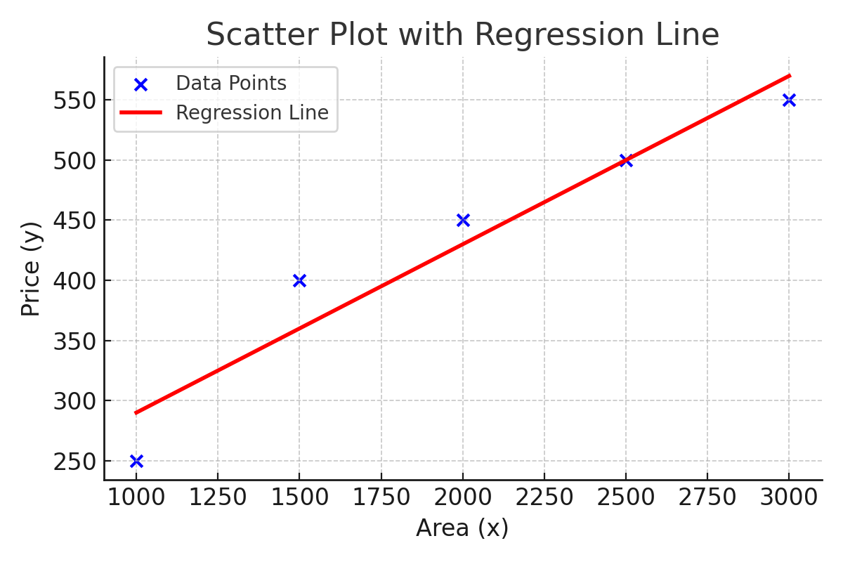
The chart below shows our five data points (blue dots) and the fitted regression line (red). Notice how the line passes through the "center" of the data, some points are above, some are below, but the line balances them. That is exactly what least squares does: minimize the total squared distance from all points to the line.
The residual plot below shows the difference between each actual price and the model's prediction. If the regression line is a good fit, the residuals should be randomly scattered around zero with no obvious pattern.
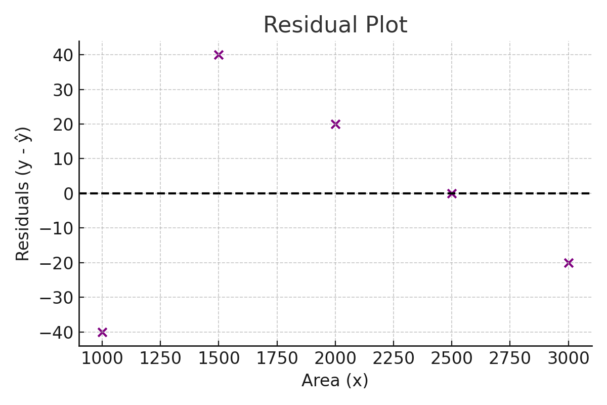
The residuals are fairly balanced, no strong pattern. This is what we want to see. Patterns in residuals (a curve, or errors growing larger as x increases) would suggest the model is missing something important about the data.
6. A Note on n vs n-1 in the Formulas
If you have studied statistics before, you may have seen variance and covariance formulas that divide by n−1 instead of n. This is called Bessel's correction and is used to get an unbiased estimate of the population variance.
However, it does not matter for the regression slope formula:
$$ \hat{\beta}_1 = \frac{\text{Cov}(x,y)}{\text{Var}(x)} $$
Whether you divide both covariance and variance by n or by n−1, the factor cancels out and the slope is the same. So you will see both conventions in textbooks, they give identical answers.
The denominator does matter when estimating the variance of the residuals (for confidence intervals and hypothesis tests):
$$ \hat{\sigma}^2 = \frac{\text{SSE}}{n-2} $$
Here, we divide by n−2 because we estimated two parameters (\(\beta_0\) and \(\beta_1\)), which "use up" two degrees of freedom.
7. Conclusion
We derived and computed the regression line from scratch. Our final equation was:
$$ \hat{y} = 150 + 0.14x $$
This is not magic, it is simply the ratio of covariance to variance, adjusted so the line passes through the mean point of the data. The slope tells you how much y changes per unit of x; the intercept is a mathematical anchor.
Once you understand simple linear regression, the extension to multiple predictors is a natural next step, the same least squares principle, applied to more variables simultaneously.
References
- Montgomery, D. C., Peck, E. A., & Vining, G. G. (2021). Introduction to Linear Regression Analysis (6th ed.). Wiley.
- Wooldridge, J. M. (2019). Introductory Econometrics: A Modern Approach (7th ed.). Cengage.
- Freedman, D., Pisani, R., & Purves, R. (2007). Statistics (4th ed.). W. W. Norton & Company.
- Gujarati, D. N., & Porter, D. C. (2009). Basic Econometrics (5th ed.). McGraw-Hill.
Related Articles