Multiple Linear Regression: A Step-by-Step Explanation
In the previous post on Simple Linear Regression, we predicted house prices using just one variable: house size. The model worked reasonably well, but in the real world, prices depend on many factors at once, size, number of bedrooms, location, age of the building, and more.
Multiple Linear Regression (MLR) extends simple regression to handle multiple predictors simultaneously. Instead of fitting a line through 2D data, we now fit a plane (with two predictors) or a hyperplane (with three or more predictors) through multi-dimensional data. The math is more involved, but the core idea, minimize squared errors, is exactly the same.
1. The Idea Behind Multiple Linear Regression
The MLR equation extends the simple regression line by adding a term for each new predictor:
\[ y = \beta_0 + \beta_1 x_1 + \beta_2 x_2 + \cdots + \beta_p x_p + \varepsilon \]
- \(y\): the outcome we want to predict (e.g., house price)
- \(x_1, x_2, \dots, x_p\): the predictors (e.g., area, bedrooms, age)
- \(\beta_0\): the intercept, baseline value when all predictors are zero
- \(\beta_j\): the coefficient for predictor \(j\), how much y changes per unit of \(x_j\), holding all other predictors constant
- \(\varepsilon\): the error term, variation we cannot explain with the predictors
The "holding others constant" interpretation is crucial. Think of cooking: suppose you want to know how much salt affects the final taste. If you also change the amount of oil and spices at the same time, you cannot isolate the effect of salt. MLR solves this problem, each coefficient tells you the effect of one ingredient while all others are held fixed.

2. How the Coefficients Are Found
The Least Squares Principle
Just as in simple regression, we find coefficients by minimizing the Sum of Squared Errors (SSE):
\[ \text{SSE} = \sum_{i=1}^n \bigl(y_i - \hat{y}_i\bigr)^2 \]
where the fitted values are:
\[ \hat{y}_i = b_0 + b_1 x_{1i} + b_2 x_{2i} \]
With one predictor, calculus gives us simple formulas. With many predictors, the algebra is best handled using matrix notation. The compact solution is:
\[ \mathbf{b} = (X^\top X)^{-1} X^\top y \]
You do not need to memorize this formula, modern software like scikit-learn handles it automatically. But knowing it exists helps you understand that MLR is still "minimize squared errors, just in higher dimensions."
For this tutorial, we will use the deviations from the mean approach, it makes the calculations more transparent.
3. Example Dataset
We will extend our house price example by adding a second predictor: number of bedrooms. Both area and bedrooms should affect price, but by how much does each one matter when we account for the other simultaneously?
| House | Area (sq.ft), x₁ | Bedrooms, x₂ | Price ($k), y |
|---|---|---|---|
| 1 | 1000 | 2 | 250 |
| 2 | 1500 | 3 | 400 |
| 3 | 2000 | 4 | 450 |
| 4 | 2500 | 3 | 500 |
| 5 | 3000 | 5 | 550 |
4. Step-by-Step Solution
Step 1: Compute the Means
Find the average of each variable. Every deviation and cross-product calculation below uses these as reference points:
\[ \bar{x}_1 = 2000, \quad \bar{x}_2 = 3.4, \quad \bar{y} = 430 \]
Step 2: Compute Deviations from the Mean
Subtract each variable's mean from its values. Deviations reveal whether each house is above or below average on each dimension.
| House | x₁ | x₁ − x̄₁ | x₂ | x₂ − x̄₂ | y | y − ȳ |
|---|---|---|---|---|---|---|
| 1 | 1000 | −1000 | 2 | −1.4 | 250 | −180 |
| 2 | 1500 | −500 | 3 | −0.4 | 400 | −30 |
| 3 | 2000 | 0 | 4 | +0.6 | 450 | +20 |
| 4 | 2500 | +500 | 3 | −0.4 | 500 | +70 |
| 5 | 3000 | +1000 | 5 | +1.6 | 550 | +120 |
House 1 is below average on all three variables: smaller, fewer bedrooms, and cheaper than typical. House 5 is above average on all three. These aligned deviations are why area and bedrooms both have positive coefficients in the final model.
Step 3: Compute Cross-Products
To solve the normal equations, we need five cross-product sums. Think of each one as measuring how two variables "move together" across the dataset.
| House | (x₁')² = Sx₁x₁ | (x₂')² = Sx₂x₂ | x₁'y' = Sx₁y | x₂'y' = Sx₂y | x₁'x₂' = Sx₁x₂ |
|---|---|---|---|---|---|
| 1 | 1,000,000 | 1.96 | 180,000 | 252 | 1400 |
| 2 | 250,000 | 0.16 | 15,000 | 12 | 200 |
| 3 | 0 | 0.36 | 0 | 12 | 0 |
| 4 | 250,000 | 0.16 | 35,000 | −28 | −200 |
| 5 | 1,000,000 | 2.56 | 120,000 | 192 | 1600 |
| Sum | 2,500,000 | 5.2 | 350,000 | 440 | 3000 |
Step 4: Set Up and Solve the Normal Equations
These sums form a system of two equations with two unknowns (\(b_1\) and \(b_2\)):
\[ 2{,}500{,}000 \, b_1 + 3000 \, b_2 = 350{,}000 \] \[ 3000 \, b_1 + 5.2 \, b_2 = 440 \]
Solving this system (using substitution or matrix methods) gives:
\[ b_1 \approx 0.125, \quad b_2 \approx 12.5 \]
Interpretation:
- Each additional square foot of area adds approximately $125 to the predicted price, holding bedrooms constant.
- Each additional bedroom adds approximately $12,500 to the predicted price, holding area constant.
Notice that the area coefficient is different from the 0.14 we found in simple regression. That is expected, adding bedrooms changes how the model credits area alone. This is the essence of MLR: each coefficient is adjusted to account for the other predictors.
Step 5: Compute the Intercept
The intercept is calculated from the means:
\[ b_0 = 430 - (0.125)(2000) - (12.5)(3.4) \approx 137.5 \]
Final regression equation:
\[ \hat{y} = 137.5 + 0.125 x_1 + 12.5 x_2 \]
Visualizing the Regression Plane
With two predictors, the fitted model is a flat surface in 3D space, not a line, but a plane. Each house is a blue dot in this 3D space, and the red plane is the model's best fit.
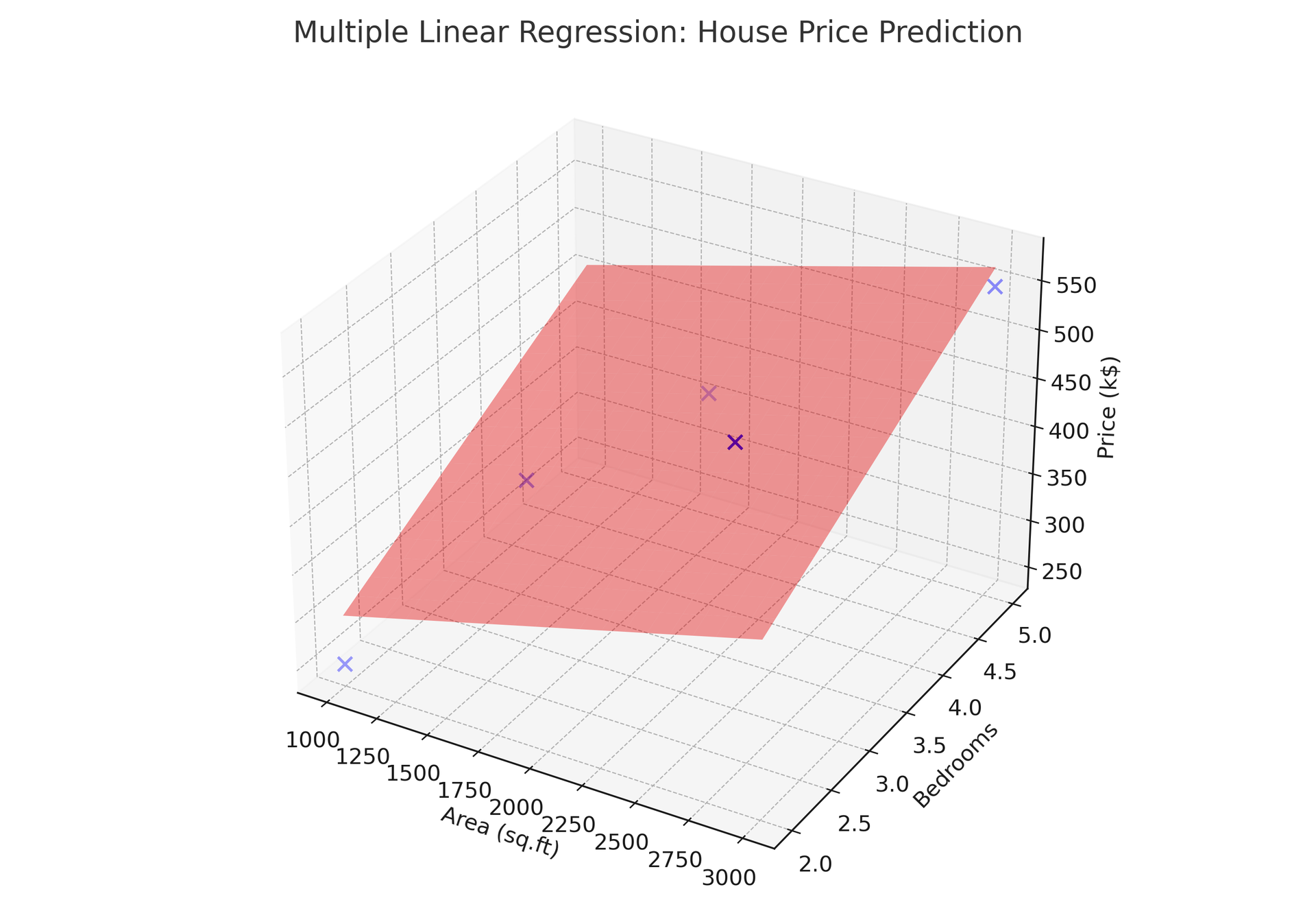
As both area and bedroom count increase, the plane rises, predicting a higher price. The plane cannot bend or curve; it is a linear model. If the true relationship curves, a linear model will be systematically off in some regions.
5. Making a Prediction
Suppose we want to predict the price of a 2,200 sq ft house with 4 bedrooms:
\[ \hat{y} = 137.5 + 0.125(2200) + 12.5(4) = 137.5 + 275 + 50 = 462.5 \text{ ($k)} \]
Our model estimates this house would cost around $462,500. This combines both the area and bedroom contributions together, something a simple regression on area alone could not do.
6. Assumptions and Pitfalls
MLR makes several assumptions. When they are violated, predictions become unreliable or misleading. Here are the key ones every beginner should know:
- Linearity, each predictor is assumed to have a straight-line effect on the outcome. If the true relationship is curved, the linear model will be systematically off.
- No multicollinearity, predictors should not be very highly correlated with each other. If area and number of rooms are almost perfectly correlated, the model cannot tell which one is doing the work, and coefficients become unstable. Think of trying to figure out which of two nearly identical ingredients changes the taste, you cannot isolate them.
- Homoscedasticity, the spread of residuals should be roughly constant across all predicted values. If large houses show much more price variability than small houses, this assumption is violated.
- Independence of observations, each data point should be independent of the others. House prices in the same neighborhood may be correlated, violating this assumption.
- Normality of residuals (for hypothesis tests), residuals should roughly follow a normal distribution if you want valid confidence intervals and p-values. For prediction accuracy alone, this assumption matters less.
Conclusion
Multiple Linear Regression extends simple regression by balancing contributions from several variables simultaneously. We walked through the derivation, solved an example by hand, and interpreted the coefficients, noting that they always have an "all else equal" meaning.
MLR is one of the most widely used tools in data science because it is transparent and interpretable. Once you are comfortable with two predictors, adding more follows the same principles. The next challenge is regularization, techniques like Ridge and Lasso that handle cases where you have too many predictors or predictors that are highly correlated.
References
- Montgomery, D.C., Peck, E.A., & Vining, G.G. (2021). Introduction to Linear Regression Analysis (6th ed.). Wiley.
- James, G., Witten, D., Hastie, T., & Tibshirani, R. (2021). An Introduction to Statistical Learning (2nd ed.). Springer (free online).
- Weisberg, S. (2005). Applied Linear Regression (3rd ed.). Wiley.
Related Articles