K-Nearest Neighbors (KNN). Part 1: Classification
Before We Start: The Core Idea in One Sentence
KNN classifies a new data point by asking: "What do the k closest points in my training data look like?", then it takes a majority vote. That's the whole algorithm. Everything else is details about how to measure "closest" and how many neighbors to ask.
1. What Is KNN?
K-Nearest Neighbors (KNN) is a classification algorithm that makes predictions without building an explicit model. Instead of learning a set of rules or weights during training, it simply remembers all the training examples and uses them at prediction time.
When you ask KNN to classify a new point, it:
- Calculates the distance from the new point to every training point.
- Picks the k training points with the smallest distances (the "nearest neighbors").
- Takes a majority vote of their labels, whatever class appears most often wins.
This style of learning, where nothing is "learned" as model parameters and the training data itself is the model, is called instance-based learning (or lazy learning).

Notice in the figure that with k=3 (inner circle), the green point gets classified as red. With k=5 (outer circle), it gets classified as blue. The choice of k genuinely changes the answer, that's why selecting it carefully matters.
2. Where the Equations Come From. Geometry + Voting
KNN uses two simple ideas: distance to measure how close points are, and voting to combine labels from neighbors into a single prediction. Both come from elementary geometry and counting.
Distance: Euclidean (Pythagoras)
You already know this from school: the straight-line distance between two points in a plane. In two dimensions, for points \(\mathbf{x}=(x_1,x_2)\) and \(\mathbf{y}=(y_1,y_2)\), it follows from the Pythagorean theorem:
Generalising to \(n\) dimensions (i.e., n features) gives the Euclidean (\(L_2\)) distance:
Intuitively: square the difference along each axis, add them all up (this gives the squared straight-line distance), then take the square root to return to the original scale.
Voting: Turning neighbors into a label
Once we have distances, we pick the \(k\) nearest neighbors of the query point \(q\), call this set \(N_k(q)\). The simplest prediction rule is majority vote (uniform weights), where the predicted class is simply whichever label appears most often:
A more flexible rule is distance-weighted voting, where closer neighbors get more say. Each neighbor contributes a weight \(w_i\):
Here \(\mathbb{1}(\cdot)\) is the indicator function, it equals 1 if the neighbor has class \(c\), and 0 otherwise. Common weight choices are:
- Uniform: \(w_i = 1\), all neighbors vote equally (reduces to majority vote).
- Inverse distance: \(w_i = \dfrac{1}{d(q,x_i) + \varepsilon}\), closer neighbors vote more strongly. The small \(\varepsilon\) avoids dividing by zero if a neighbor is at distance 0.
- Gaussian: \(w_i = \exp\big(-d(q,x_i)^2/(2\sigma^2)\big)\), a smooth bell-shaped decay with distance.
3. Step-by-Step Calculation
Let's work through a tiny 2D example so you can verify every step on paper. We have 5 training points and one unknown query point.
| ID | x | y | Class |
|---|---|---|---|
| P1 | 1 | 1 | A |
| P2 | 2 | 1 | A |
| P3 | 4 | 3 | B |
| P4 | 5 | 4 | B |
| P5 | 1 | 3 | A |
Query point: \(Q=(3,2)\). We want to know: should Q be classified as A or B?
Step 1. Compute distances to every training point
- \(d(Q,P1)=\sqrt{(3-1)^2+(2-1)^2}=\sqrt{4+1}=\sqrt{5}\approx 2.236\)
- \(d(Q,P2)=\sqrt{(3-2)^2+(2-1)^2}=\sqrt{1+1}=\sqrt{2}\approx 1.414\)
- \(d(Q,P3)=\sqrt{(3-4)^2+(2-3)^2}=\sqrt{1+1}=\sqrt{2}\approx 1.414\)
- \(d(Q,P4)=\sqrt{(3-5)^2+(2-4)^2}=\sqrt{4+4}=\sqrt{8}\approx 2.828\)
- \(d(Q,P5)=\sqrt{(3-1)^2+(2-3)^2}=\sqrt{4+1}=\sqrt{5}\approx 2.236\)
Step 2. Sort by distance (closest first)
| Point | Class | Distance |
|---|---|---|
| P2 | A | \(\sqrt{2}\approx 1.414\) |
| P3 | B | \(\sqrt{2}\approx 1.414\) |
| P1 | A | \(\sqrt{5}\approx 2.236\) |
| P5 | A | \(\sqrt{5}\approx 2.236\) |
| P4 | B | \(\sqrt{8}\approx 2.828\) |
4. Choose k and Predict (Manual Voting)
Pick \(k=3\). The three nearest neighbours are P2 (A), P3 (B), and P1 (A). Counting votes: A: 2, B: 1, so KNN predicts class A for Q.
Why does k matter? Ties and the odd-k trick
If we had chosen \(k=2\), we'd have P2 (A) and P3 (B), a perfect tie. Common tie-breaking strategies:
- Choose the label of the single closest neighbor (1-NN fallback).
- Use distance-weighted voting so nearer neighbors break ties naturally.
- Always use an odd k for binary classification problems to avoid ties entirely.
Distance-weighted voting (concrete numbers)
Using inverse-distance weights \(w_i=1/(d_i+\varepsilon)\) with \(\varepsilon=10^{-6}\) on the k=3 neighbors:
- \(w_{P2}=1/\sqrt{2}\approx 0.707\) (class A)
- \(w_{P3}=1/\sqrt{2}\approx 0.707\) (class B)
- \(w_{P1}=1/\sqrt{5}\approx 0.447\) (class A)
Weighted totals: A = 0.707 + 0.447 = 1.154; B = 0.707. Class A still wins, and the margin is clearer than the 2–1 majority vote.
5. Visual Illustration
The figure below shows our five training points and the query point Q(3,2). Points from class A are shown in red and class B in blue. The dashed circle marks the boundary that contains the three nearest neighbors (k = 3).
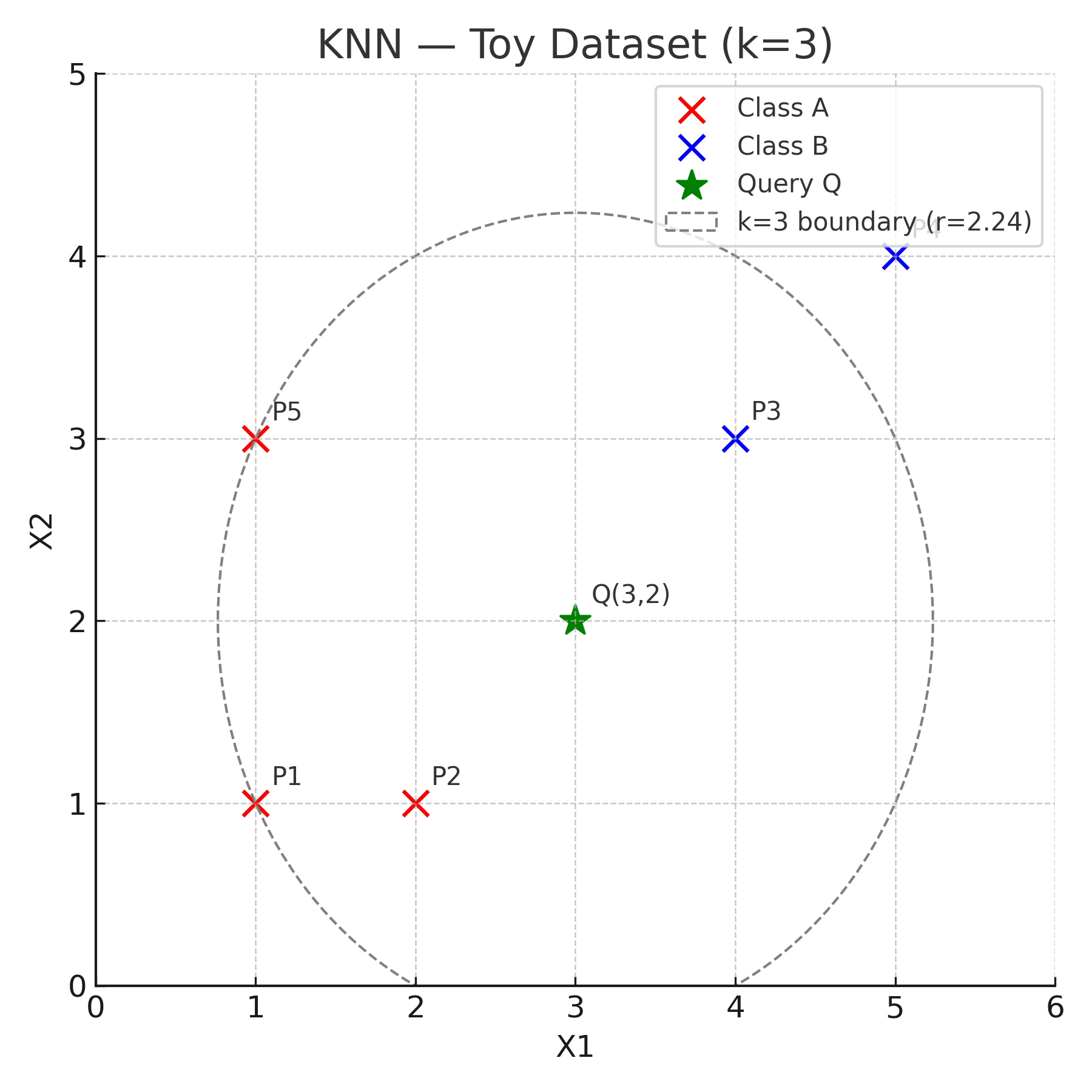
How to read this visual, look for three things:
- Which points are nearest to Q: P2 and P3 are equally close (√2 ≈ 1.414), P1 is next (√5 ≈ 2.236).
- The k=3 circle (dashed): any point inside the circle is among the 3 nearest neighbours of Q.
- Majority vote: two of the 3 neighbours are class A, so the predicted label for Q is A.
6. Practical Notes. What Can Go Wrong
- Scale your features first: KNN uses raw distances. If one feature is measured in thousands (e.g., income) and another in single digits (e.g., age on a 1–5 scale), the large-valued feature will dominate every distance calculation. Always standardize or normalize features before applying KNN.
- Pick k with cross-validation: Small k (e.g., k=1) means the model is very sensitive to individual training points, a single noisy example can swing the prediction. Large k means the model averages over more neighbors and becomes smoother, but may miss local patterns. Use k-fold cross-validation to find the best k for your data.
- Consider distance-weighted voting: Inverse-distance or Gaussian weights often help when the training data is noisy, because distant neighbors have less influence on the result.
- Distance metric is not one-size-fits-all: Euclidean (L2) is the default, but Manhattan (L1) works better when features are on very different scales, Mahalanobis accounts for feature correlations, and cosine similarity is better for text or high-dimensional sparse data.
- Beware the curse of dimensionality: In high-dimensional spaces (many features), all points become roughly equidistant from each other, the concept of "nearest neighbor" breaks down. Consider PCA or feature selection to reduce dimensions first.
7. Complexity and Scaling Up
The simplest ("naïve") implementation computes distances to all n training points for each query, that's \(O(n)\) per query. For large datasets this becomes slow.
Faster alternatives:
- KDTree / BallTree (available in scikit-learn): organize training points into a tree structure, enabling sub-linear query times in moderate dimensions.
- Approximate Nearest Neighbor (ANN) libraries like Annoy or FAISS: trade a tiny bit of accuracy for massive speed gains on millions of high-dimensional points.
8. Manual Python Calculation
This code replicates every step we did by hand, useful for building intuition before moving to a library.
import math
points = {'P1':((1,1),'A'),'P2':((2,1),'A'),'P3':((4,3),'B'),'P4':((5,4),'B'),'P5':((1,3),'A')}
Q = (3,2)

results = []
for name,(coords,label) in points.items():
    dx = Q[0] - coords[0]
    dy = Q[1] - coords[1]
    d = math.sqrt(dx*dx + dy*dy)
    results.append((name, coords, label, d))

results_sorted = sorted(results, key=lambda x: x[3])
print('Sorted neighbours:')
for r in results_sorted:
    print(r)

k = 3
neighbors = results_sorted[:k]
votes = {}
for name,coords,label,d in neighbors:
    votes[label] = votes.get(label,0) + 1
print('\nVotes (majority):', votes)

# weighted votes
w_votes = {}
for name,coords,label,d in neighbors:
    w = 1.0 / (d + 1e-9)
    w_votes[label] = w_votes.get(label, 0) + w
print('Weighted votes:', {k: round(v,3) for k,v in w_votes.items()})

print('\nFinal prediction (majority):', max(votes.items(), key=lambda x: x[1])[0])
9. Using scikit-learn (Real Projects)
In practice, use scikit-learn's KNeighborsClassifier. It handles distance computation, tie-breaking, and weighting efficiently, and integrates with pipelines for scaling.
from sklearn.neighbors import KNeighborsClassifier
import numpy as np
X = np.array([[1,1],[2,1],[4,3],[5,4],[1,3]])
y = np.array(['A','A','B','B','A'])
knn = KNeighborsClassifier(n_neighbors=3)
knn.fit(X,y)
print('Prediction for Q:', knn.predict([[3,2]])[0])
10. Key Takeaways
KNN is one of the most transparent algorithms in machine learning, you can trace every prediction back to specific training examples. The three knobs that control its behavior are:
- k, how many neighbors to consult. Too small: overfits to noise. Too large: misses local patterns. Use cross-validation to choose.
- Distance metric. Euclidean is the default, but it's not always right. Match the metric to the nature of your features.
- Weighting, uniform (majority vote) or distance-weighted. Weighted voting is more robust when neighbors vary in how close they are.
For real data: always scale your features, visualize when possible, and validate k using cross-validation. KNN is an excellent baseline before trying more complex models.
References
- Cover, T., & Hart, P. (1967). Nearest neighbor pattern classification. IEEE Transactions on Information Theory, 13(1), 21–27.
- Fix, E., & Hodges, J. L. (1951). Discriminatory Analysis, Nonparametric Discrimination: Consistency Properties. USAF School of Aviation Medicine Technical Report.
- Hastie, T., Tibshirani, R., & Friedman, J. (2009). The Elements of Statistical Learning (2nd ed.). Springer.
- Scikit-learn: Nearest Neighbors
- Voronoi diagram (visual intuition for KNN decision boundaries)