A Beginner's Guide to Lasso Regression
1. Introduction
In the previous post, we saw how Ridge Regression shrinks all coefficients toward zero to prevent overfitting. Ridge is great for stability, but it has one limitation: it never removes any feature completely. All coefficients end up small but non-zero, which means the model still uses every predictor, even irrelevant ones.
Lasso Regression (short for Least Absolute Shrinkage and Selection Operator) takes regularization one step further: it can drive some coefficients to exactly zero, effectively removing those features from the model entirely. This makes Lasso a tool for both regularization and automatic feature selection.
If you have 100 potential predictors and suspect only 10 of them truly matter, Lasso will often find those 10 and set the rest to zero, leaving you with a simpler, more interpretable model.
2. The Lasso Cost Function
To understand what makes Lasso different, compare the three loss functions side by side:
Ordinary Least Squares (OLS), minimize prediction error only:
$$ J(\beta) = \sum_{i=1}^{n} (y_i - \hat{y}_i)^2 $$
Ridge, adds an L2 penalty (sum of squared coefficients):
$$ J_{\text{ridge}}(\beta) = \sum_{i=1}^{n} (y_i - \hat{y}_i)^2 + \lambda \sum_{j=1}^p \beta_j^2 $$
Lasso, adds an L1 penalty (sum of absolute values of coefficients):
$$ J_{\text{lasso}}(\beta) = \sum_{i=1}^{n} (y_i - \hat{y}_i)^2 + \lambda \sum_{j=1}^p |\beta_j| $$
The only difference between Ridge and Lasso is whether you square the coefficients (\(\beta_j^2\)) or take their absolute values (\(|\beta_j|\)). That one change has a dramatic effect on the solution.
3. Why Does Lasso Set Coefficients to Zero?
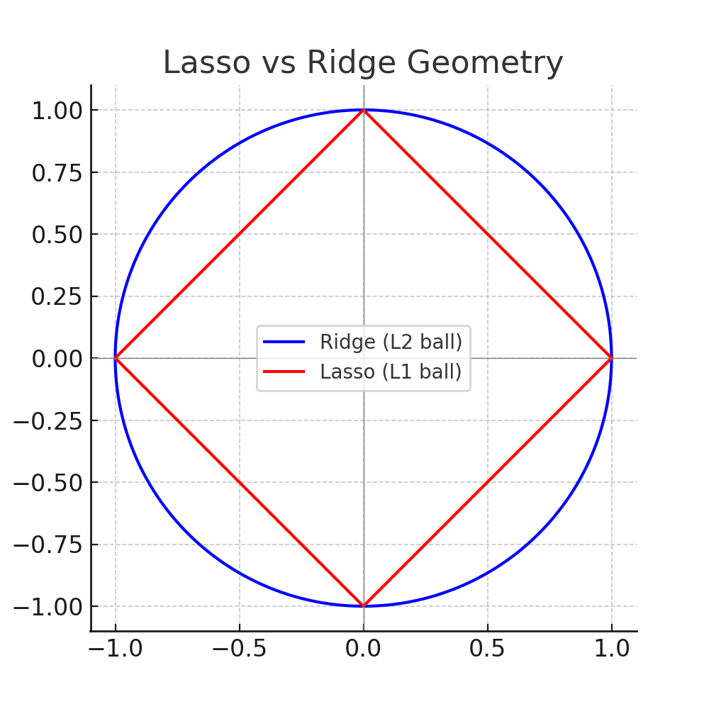
The geometric explanation is the most intuitive. Think of the cost function as a set of concentric ellipses centered on the OLS solution (the unconstrained best fit). The penalty is a constraint region, a shape that limits how large the coefficients can be. The solution must sit inside this region.
- Ridge's constraint region is a circle (smooth, curved everywhere).
- Lasso's constraint region is a diamond (four corners where axes are touched).
When the error ellipses expand outward from the OLS solution until they first touch the constraint region, they almost always touch a smooth part of the Ridge circle, giving a solution where both coefficients are non-zero. But the Lasso diamond has sharp corners right on the axes. The ellipses tend to hit these corners first, giving a solution where one coefficient is exactly zero.
In simple terms: Ridge has no corners, Lasso does, and those corners force coefficients to zero.

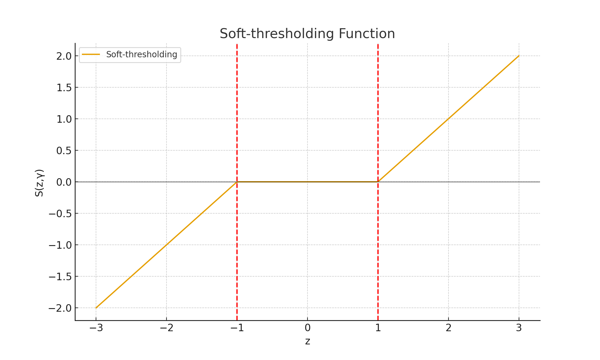
Soft-Thresholding: The Math Behind Sparsity
Lasso's solutions are computed using a technique called soft-thresholding. For each coefficient, the update rule is:
$$ S(z, \gamma) = \text{sign}(z) \cdot \max(|z| - \gamma, 0) $$
Here is what this means in plain English:
- If the raw coefficient
zis smaller than the thresholdγ, it is set to exactly zero. - If
zis larger thanγ, it is reduced byγ(shrunk toward zero, but not to zero).
This "push-to-zero" behavior is what makes Lasso a feature selector, not just a shrinker.
4. Example with a Tiny Dataset
Let us trace through the soft-thresholding steps manually on a simple four-point dataset:
| X | y |
|---|---|
| 1 | 2 |
| 2 | 3 |
| 3 | 5 |
| 4 | 7 |
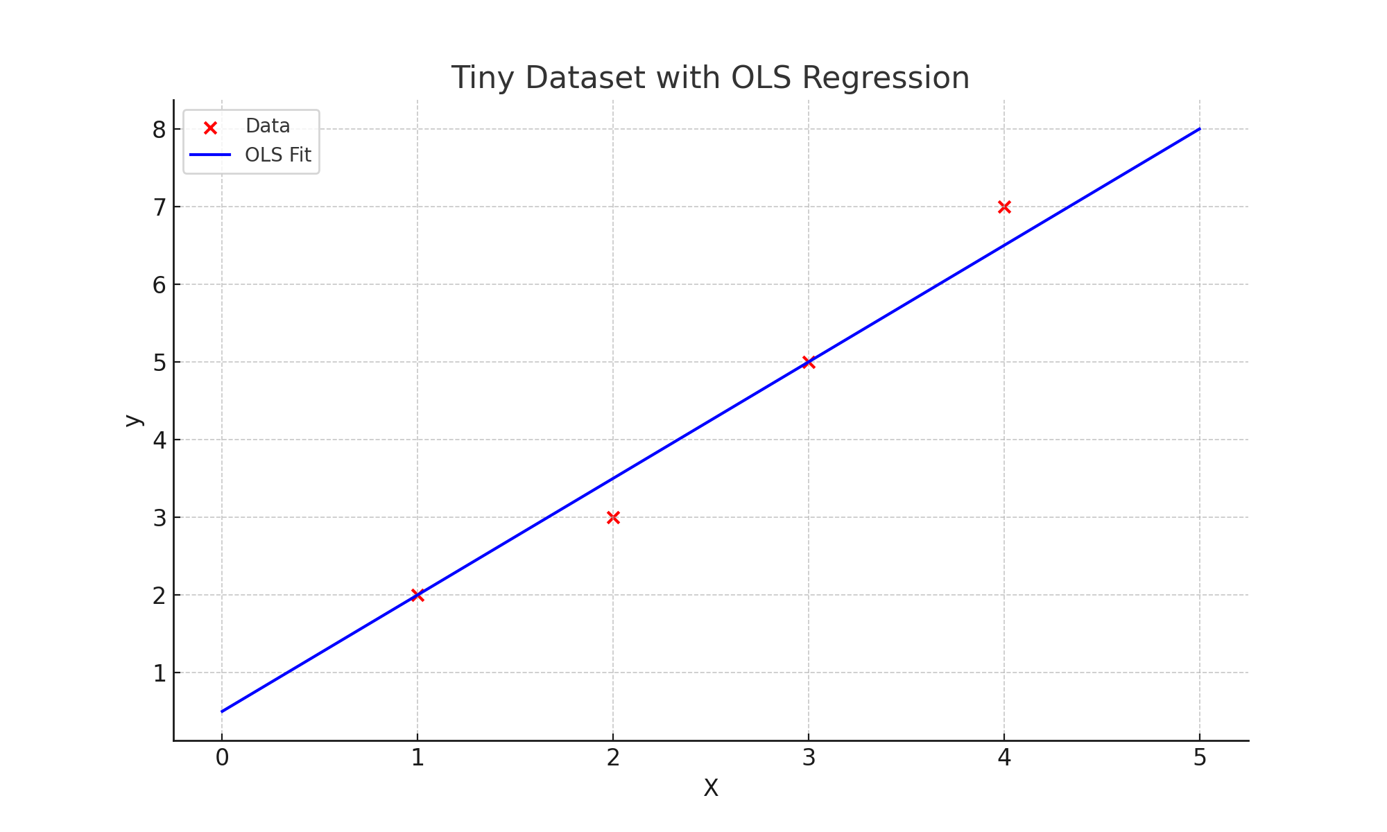
The OLS solution (without regularization) gives approximately:
$$ \hat{y} = 0.5 + 1.5x $$
Now let us apply Lasso with \(\lambda = 1\). In the simplified single-feature case:
Step 1: Compute the raw correlation z
$$ z = \frac{1}{n} \sum x_i y_i = \frac{1}{4}(1 \times 2 + 2 \times 3 + 3 \times 5 + 4 \times 7) = 12.75 $$
Step 2: Compute the threshold γ
$$ \gamma = \frac{\lambda}{2n} = \frac{1}{8} = 0.125 $$
Step 3: Apply soft-thresholding
$$ \beta_1 = S(12.75,\ 0.125) = 12.75 - 0.125 = 12.625 $$
The coefficient shrinks slightly from 12.75 to 12.625. If we had used a larger \(\lambda\), the threshold would be larger and the shrinkage more dramatic. At some point, \(z\) would be smaller than \(\gamma\) and the coefficient would collapse to exactly zero.
Important note on scale: The value 12.625 is the result of a single coordinate-descent sub-step applied to the raw (unnormalized) dot product \(z = \frac{1}{n}\sum x_i y_i\). It is not a fitted slope coefficient in the usual sense and should not be compared directly to the OLS slope of approximately 1.5. The OLS slope is derived from the standard formula that accounts for the variance of \(x\), whereas \(z\) here is an intermediate quantity in the soft-thresholding calculation. This example illustrates the soft-thresholding operator in isolation, not a complete Lasso model fit.
Step 4: Manual Python Demo
import numpy as np

X = np.array([1,2,3,4])
y = np.array([2,3,5,7])
n = len(y)

# Compute raw correlation
z = (1/n) * np.sum(X * y)
lam = 1
gamma = lam / (2*n)   # soft-threshold value

def soft_threshold(z, gamma):
    if z > gamma:
        return z - gamma
    elif z < -gamma:
        return z + gamma
    else:
        return 0   # coefficient set to zero

beta1 = soft_threshold(z, gamma)
print("z =", z)           # 12.75
print("gamma =", gamma)   # 0.125
print("Updated coefficient β1 =", beta1)   # 12.625
print("Predictions:", beta1 * X)
5. Using Scikit-learn
In practice, Lasso is optimized iteratively (coordinate descent) because the absolute value function is not differentiable at zero. Scikit-learn handles all of this for you:
from sklearn.linear_model import Lasso
import numpy as np
from sklearn.preprocessing import StandardScaler

X = np.array([[1],[2],[3],[4]])
y = np.array([2,3,5,7])

# Always standardize before Lasso, the penalty is scale-sensitive
scaler = StandardScaler()
X_scaled = scaler.fit_transform(X)

model = Lasso(alpha=1)   # alpha = lambda
model.fit(X_scaled, y)

print("Intercept:", model.intercept_)
print("Coefficient:", model.coef_)
Notice that with a large enough alpha, the coefficient will print as exactly 0.0,
Lasso has removed that feature from the model. This is the feature selection in action.
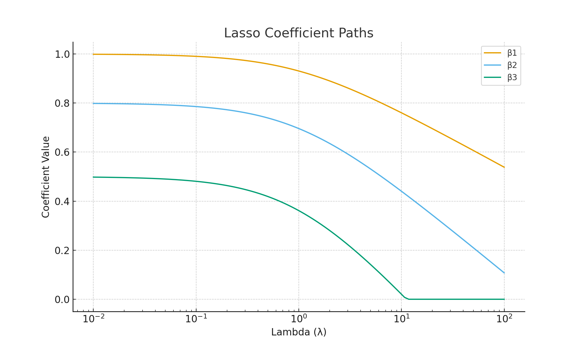
6. Regularization Path
A regularization path shows how each coefficient changes as \(\lambda\) increases. For Lasso, some coefficients reach zero and stay there, those features are eliminated. Features that survive longest (coefficients reaching zero at high \(\lambda\)) are the most important predictors.
7. Ridge vs Lasso: A Quick Comparison
| Aspect | Ridge (L2) | Lasso (L1) |
|---|---|---|
| Penalty type | Squared coefficients (\(\beta_j^2\)) | Absolute coefficients (\(|\beta_j|\)) |
| Constraint shape | Circle (smooth) | Diamond (sharp corners) |
| Coefficients reach zero? | No, only shrinks | Yes, can eliminate features |
| Best for | Correlated predictors, stability | Feature selection, sparse models |
| When predictors are correlated | Keeps all, shrinks all | Arbitrarily picks one, zeroes others |
When predictors are correlated, Lasso tends to arbitrarily pick one and discard the others, which can be unstable. In that case, Elastic Net (covered in the next post) combines both penalties to get the best of both approaches.
8. Key Takeaways
- Lasso uses an L1 penalty (absolute values), which can drive coefficients to exactly zero, performing automatic feature selection.
- Ridge uses L2 (squared values), which only shrinks coefficients, never eliminating them.
- Always standardize features before applying Lasso, the L1 penalty is scale-sensitive, and features on larger scales will be unfairly penalized.
- The choice of \(\lambda\) (called
alphain scikit-learn) is critical: too small → overfitting, too large → underfitting. Use cross-validation to tune it. - When you have many features and expect most to be irrelevant, Lasso is often the first regularization method to try.
9. Conclusion
Lasso is a powerful tool that does two jobs at once: it reduces overfitting through regularization, and it simplifies models by automatically removing irrelevant predictors. The key intuition: Ridge shrinks, Lasso selects. Use Ridge when you want stability and all features matter; use Lasso when you suspect many features are irrelevant and want a cleaner model.
References
- Tibshirani, R. (1996). Regression Shrinkage and Selection via the Lasso. Journal of the Royal Statistical Society, Series B, 58(1), 267–288.
- Hoerl, A. E., & Kennard, R. W. (1970). Ridge Regression: Biased Estimation for Nonorthogonal Problems. Technometrics, 12(1), 55–67.
- Hastie, T., Tibshirani, R., & Friedman, J. (2009). The Elements of Statistical Learning (2nd ed.). Springer.
- Scikit-learn. Lasso Documentation
- Zou, H., & Hastie, T. (2005). Regularization and variable selection via the elastic net. Journal of the Royal Statistical Society, Series B, 67(2), 301–320.
Related Articles